10 EJ - Drawing Polygons for Warehouse downzoning in Mead Valley

Today we will focus on the practice of creating polygons for use in a warehouse mapping visualization.

There is an unincorporated community in the County of Riverside called Mead Valley that has about 20,000 residents that has among the highest concentration of warehouse space per capita of any place in the Inland Empire. Here is some census info on Mead Valley.

The County is currently undergoing an 8-year planning cycle to amend the General Plan for land use called the Foundation Amendment Cycle.

I want to make a map to show all the planned changes and indicate how the area is going to change. Also, I’d like us to update the wiki page on Mead Valley.

10.1 Existing Conditions

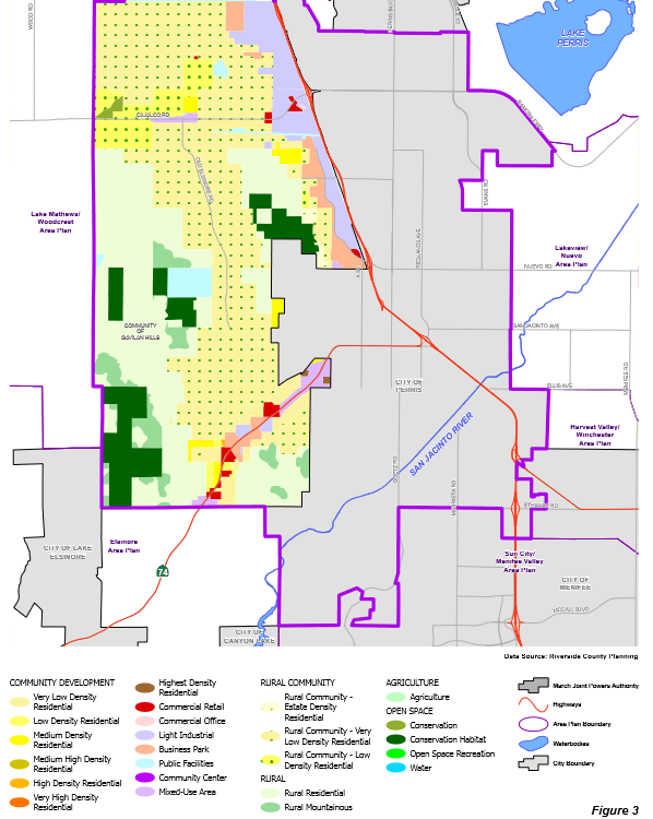
The Mead Valley Area Plan is part of the Riverside County General Plan. A picture of the land use planning is shown in that document in Figure 3, reproduced here.

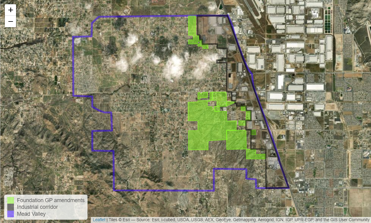
Mead Valley Area Plan Industrial development is focused around the 215 freeway corridor to the East of the Mead Valley Planning area.

Let’s poke around Warehouse CITY to get a sense of the current development and future development.

Notice that the adjacent unincorporated communities of Woodcrest and Lake Mathews have zero warehouses - they are majority white communities.

10.2 Cumulative Impacts

Today, I am going to ask you all to help with a cumulative impacts analysis for understand the cumulative impacts of the Foundation Amendments. Under CEQA Section 15355, cumulative impacts are defined as ‘two or more individual effects, when considered together, are considerable or which compound or increase other environmental impacts…The cumulative impact from several projects is the change in the environment which results from the incremental impact of the project when added to other closely related past, present, and reasonably foreseeable future projects.’

A cumulative impacts analysis identifies the past, present, and probable future projects that should be included in environmental analysis.

In Spring 2023, my class helped add dozens of planned warehouses to the existing warehouses map. This work helped us to add a layer of ’planned and approved warehouses to the tool allowing users to see what warehouses are likely to be built in the near future.

In this class, I hope to assess the cumulative impacts of the General Plan amendments to the Mead Valley community to answer three key questions and illustrate them using an environmental data visualization to submit as public comment to the County (planning commission and Board of Supervisors).

How are land uses shifting (e.g., from residential to industrial)?
What is the spatial pattern of shifting land-use?
How much land is lost for housing (acres and dwelling units)?

10.3 Visualization - Drawing a Polygon

We’re going to draw some polygons. Just like in our first spatial visualization lecture, we’re going to identify latitude and longitude pairs for the vertices of the polygon. However, we’ll run a couple of sf functions on them to transform the individual numbers into a simple features polygon.

Note, this is a highly manual approach. There are better ways to do this systematically and I’ve developed a tool to start doing that called the Polygon Export Tool. I will show you how to use that in the next unit, because it requires importing data.

First, we do the most basic way. After that, we’ll show the tool and how it can simplify the process - assuming you know where to find files on your machine.

10.3.1 Load libraries

library(sf)
library(leaflet)
library(dplyr)

10.3.2 Manually Identify the Polygon Vertices.

Open Google Maps or an equivalent mapping tool with satellite imagery and an ability to click on a location and retrieve a decimal degree location.

Find a vertex on the map - input longitude and latitude into a list in the form c(lng, lat).

Do that for all the vertex points and bind them together as a list of lists as shown in the code below.

Let’s do that for the boundary of Mead Valley.

MeadValley <- rbind(
                    c(-117.319618, 33.865782),
                    c(-117.261695, 33.86626),
                    c(-117.23327, 33.8012),
                    c(-117.24842, 33.80129),
                    c(-117.24842, 33.804726),
                    c(-117.25254, 33.804726),
                    c(-117.25254, 33.80829),
                    c(-117.26752, 33.80829),
                    c(-117.26752, 33.80025),
                    c(-117.31279, 33.80025),
                    c(-117.31279, 33.82981),
                    c(-117.32242, 33.83189),
                    c(-117.32242, 33.83561),
                    c(-117.33111, 33.83595),
                    c(-117.33111, 33.85819),
                    c(-117.32265, 33.8584),
                    c(-117.32267, 33.86331),
                    c(-117.319618, 33.865782)
                    )

Look at the MeadValley table in your Environment panel - it looks like a table of point coordinates.

We need one more bit of code to convert that into a polygon. It is complicated.

MeadValleyPoly <- st_sf(
                      name = 'Mead Valley', 
                      geom = st_sfc(st_polygon(list(MeadValley))), 
                      crs = 4326
                      )

The name is our label for the polygon, so that’s easy. The crs is the coordinate reference system, in this case WGS84 = 4326 for easy display in leaflet.

The geom is the geometry. Three functions are applied - list() which converts the MeadValley table to a list, st_polygon() which returns a polygon from a list of coordinates, and st_sfc() which verifies the contents and sets its class.

Polygons always have to start and end with the same vertex to be a closed loop.

Now we should display it to make sure it looks correct. Figure 10.1 shows the polygon with a basic map.

leaflet()  |>  
  addTiles() |> 
  addPolygons(data = MeadValleyPoly)

Figure 10.1: Mead Valley Polygon Check

That looks pretty good, although I skipped a couple of wiggles.

Now let’s do a modification of the basic map using addPolylines() instead of addPolygons() and showing you how to add a few warehouses.

Now let’s add a warehouse layer showing all planned and approved warehouse projects within California that went through CEQA review from 2020-2024.

First import the warehouse dataset. Let’s name this dataset warehouses, just like we did in 8.3.2.2.

WH.url <- 'https://raw.githubusercontent.com/RadicalResearchLLC/WarehouseMap/main/WarehouseCITY/geoJSON/comboFinal.geojson'
warehouses <- st_read(WH.url) |>  
  st_transform(crs = 4326) |> 
  filter(county == 'Riverside County')

Reading layer `comboFinal' from data source 
  `https://raw.githubusercontent.com/RadicalResearchLLC/WarehouseMap/main/WarehouseCITY/geoJSON/comboFinal.geojson' 
  using driver `GeoJSON'
Simple feature collection with 9106 features and 8 fields
Geometry type: MULTIPOLYGON
Dimension:     XY
Bounding box:  xmin: -118.8037 ymin: 33.43325 xmax: -114.4085 ymax: 35.55527
Geodetic CRS:  WGS 84

Now let’s add the existing warehouses to the map.

Figure 10.2

palWH <- colorFactor(palette = c('darkred', 'orange', 'black'),
                     domain = warehouses$category)

leaflet() |> 
  addTiles() |> 
  addPolylines(data = MeadValleyPoly,
              color = 'blue',
              weight = 3) |> 
  addPolygons(data = warehouses,
              color = ~palWH(category),
              weight = 1)

Figure 10.2: Mead Valley warehouses in bigger context with less busy map.

It is a map, but the zoom level is not focused on the salient part we’re interested in. We can use the setView() function to set the zoom level. We showed an example of this in lesson 3.

Figure 10.3

leaflet() |> 
  addTiles() |> 
  addPolylines(data = MeadValleyPoly,
              color = 'blue',
              weight = 3) |> 
  addPolygons(data = warehouses,
              color = ~palWH(category),
              weight = 1) |> 
  setView(zoom = 12, lat = 33.85, lng = -117.2) ## Add zoom level and map center point

Figure 10.3: Mead Valley warehouses zoomed just to the local area.

This is better, but I want a better underlying tile view. We can use the addProviderTiles() function to replace addTiles() to get a different underlying tile map. Here we will add the Esri.WorldImagery layer to see the satellite view.

Figure 10.4

leaflet() |> 
  addProviderTiles(provider = providers$Esri.WorldImagery) |> ## We modified this line to change to satellite view  
  addPolylines(data = MeadValleyPoly,
              color = 'blue',
              weight = 3) |> 
  addPolygons(data = warehouses,
              color = ~palWH(category),
              weight = 1,
              fillOpacity = 0.6) |> 
  addLegend(data = warehouses,
            pal = palWH,
            values = ~category) |> 
  setView(zoom = 12, lat = 33.85, lng = -117.25)

Figure 10.4: Mead Valley warehouses zoomed just to the local area with a satellite image tile map

10.3.3 Existing Conditions

I went to Riverside County Mapping Portal to download the industrial zoned parcels in Mead Valley. The Boundaries & Sites url has the data that can be used to filter the dataset down to the information needed to create the map.
I used my polygon export tool to draw maps for each General Plan Amendment proposed that is light-industrial or business park. There aren’t enough details to show where building parcels will go and two of the projects are reserving some space for other uses (open space or residential).

10.3.4 Planned Warehouses map for Mead Valley Foundation plan amendments

Figure 10.5

Figure 10.6

10.1 Existing Conditions

10.2 Cumulative Impacts

10.3 Visualization - Drawing a Polygon

10.3.1 Load libraries

10.3.2 Manually Identify the Polygon Vertices.

10.3.3 Existing Conditions

10.3.4 Planned Warehouses map for Mead Valley Foundation plan amendments

10.3.5 Planned Warehouses Map with Major Planned Roadway Widenings