25 Data Import - Theory and Practice
This lecture provides a systematic overview of key steps in the acquisition and import of data.
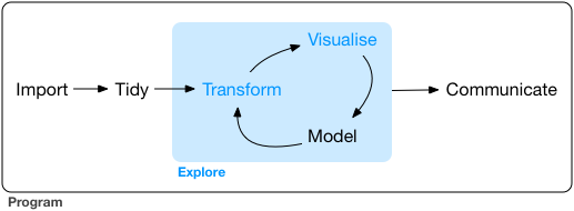
As a reminder, our framework for the workflow of data visualization is shown in Figure 25.1
25.1 Overview
- Clearly define the research question
- Identify relevant authoritative data sources
- Critically evaluate the data sources
- Import the data
- Review and tidy the data
Some sources to peruse for more information on data import using R.
- R for Data Science 2e - Data Import
- An Introduction to R - Data
- Reading, Writing and Converting Simple Features
- Introduction to Data Science - Importing Data
25.1.1 Step 0. Clearly define the question or objective
The zeroeth step is to identify what it is you are planning to do. Delineat the scope of the project for the purposes of defining the data needs.
- Spatial extent
- Temporal extent
- Variables/parameters (environmental variables, socioeconomic information, categorical information, jurisdictions)
25.1.1.1 Example - Particulate emissions sources affecting Fontana and Bloomington
- Spatial extent - The city of Fontana and the census designated place of Bloomington boundaries with a 1 km buffer
- Temporal extent - Emissions sources operational as of 2020 or later.
- Variables/parameters - Major roads, local roads, rail, railyards, industrial facilities in emissions inventory, small area sources like gas stations, restaurants, truck terminals, and warehouses
- DQOs - authoritative sources (census, government agency datasets, OpenStreetMaps, Peer Reviewed Data Products)
25.1.1.2 Example - Road widening projects in Riverside County and induced Freight VMT/demand
- Spatial extent - Western Riverside County - west of Banning
- Temporal extent - Projects constructed between 2014-2024 and planned through 2030
- Variables/parameters - Road links, vehicle and truck AADT, warehouse land-use, residential developments
25.1.3 Step 2. Critically evaluate the data sources
Prior to acquiring the data, it is important to evaluate its utility for your goals, to the extent possible.
- What type of data is it? (geospatial, tabular, categorical, qualitative)
- Does it cover the spatial domain?
- Is it the right temporal period?
- Does it have the right variables?
- What format is it in?
- Does it require any specific citations, licenses, and/or attribution for use?
Sometimes these things can’t be evaluated until you import the data. Iterate through step 2-4 as needed.
25.1.3.1 Example - PM emissions
The tigris package is a wealth of primary authoritative data. - roads() data is authoritative, recent, spatially comprehensive, geospatial data. ✅
- rails() data - same as roads, but does require some spatial tidying. ✅ - places() data - usable to zoom in on spatial scope - requires some spatial tidying/buffering. ✅
US EPA data for National emissions inventory - this has location information for large sources. ✅
SCAQMD data for source magnitudes from PM AQMP, see table and links to primary sources. ✅
Restaurant data - I haven’t found a good source for tabular and spatial data on restaurants. Google API might work but requires registration.
25.1.3.2 Example - Roads
RCTC website has project information, but it isn’t directly downloadable/scrapable. Tidying required. ✅
The tigris package is a wealth of primary authoritative data. - roads() data is authoritative, recent, spatially comprehensive, geospatial data. ✅
Caltrans open data has point data for AADT and truck AADT. Will require spatial joins to road links. Single year of data. Spreadsheets contain multiple years that can be linked to this.
Riverside County open data has zoning polygons for identifying residential areas, but not necessarily new areas. Other municipalities may be needed to cover specific road segments.
25.1.4 Step 3. Import Data
3.1 Identify the data format 3.2 Can I scrape it directly? Is there a url or API or a package in R that will allow me to scrape it? If so, that’s probably the best choice for a reproducible workflow. Examples include tidycensus, tigris, warehouses, co2, and SoCalEJ datasets. 3.3 If not, download it.
3.3a - Unzip it if zipped or compressed. 3.3b - move data to working directory or point import script to location it is stored. Keeping data in a specific working directory is a better practice.
3.4 - Import it using appropriate function (st_read(), read_table(), read_csv(), etc.) 3.5 - Review data import 3.5a - look at data table 3.5b - make a basic visualization
25.1.4.1 Example - PM emissions
Scrape roads(), rails(), and places() and warehouses.
Import facility data from F.I.N.D tool at SCAQMD using openxlsx::read.xlsx().
Google maps api call for restaurants or manually assemble restaurant list - both could be slow and painful.
25.1.4.2 Example - Roads
Scrape roads() and warehouses.
Download passenger and truck AADT data from Caltrans.
Residential zoning is available for the county and potentially some municipalities for download.
Assemble road widening project data from county website into data table(s).
25.1.5 Step 4. Review and tidy data.
Use head(), tail(), to examine imported rows.
- Check that the number of records seems reasonable - a zero record import is usually bad
- Check for column names, and check that they are R friendly (avoid spaces, special characters)
- Check column types - common errors include dates imported as character types or other incorrect assignments.
- Check for
NAand null records, rows, and columns. - For geospatial data - check coordinate reference system
As necessary, tidy the data to get it in the form you need. See all the data science steps in Data Science 101